41 excel pivot table labels

Use column labels from an Excel table as the rows in a ... Close the dialog and keep the changes. Excel should place the unpivoted data into a new worksheet, looking something like this: Now the final step is to create a pivot table using this unpivoted data. Here is a screenshot of my pivot table setup: Note that Attribute (e.g. Malaria, Tuberculosis) is placed above the Year. This lets us open or ... Turn Repeating Item Labels On and Off - Excel Pivot Tables Select a cell in the pivot field that you want to change On the PIVOT POWER Ribbon tab, in the Pivot Items group, click Show/Hide Items Click Repeat Item Labels - On or Repeat Item Labels - Off To set the Default Setting: On the PIVOT POWER Ribbon tab, in the Formatting group, click Set Defaults

Changing Blank Row Labels - Excel Pivot Tables You can manually change the (blank) labels in the Row or Column Labels areas by typing over them in the pivot table. You can type any text to replace the (Blank) entry, but you can't clear the cell and leave it empty: Select one of the Row or Column Labels that contains the text (blank). Type N/A in the cell, and then press the Enter key.

Excel pivot table labels

Microsoft Excel - showing field names as headings rather ... In earlier versions, by default if you create a pivot table, instead of showing the field names, it will say row labels and column labels. To see the field names instead, click on the Pivot Table Tools Design tab, then in the Layout group, click the Report Layout dropdown and select either Show in Outline Form or Show in Tabular form. Change the pivot table "Row Labels" text | MrExcel Message ... Feb 4, 2021. #3. mart37 said: Click on the cell and typ the text. Click to expand... Thanks mart37. So simple! I was looking for a way to change it on the ribbons & settings. Typical Excel - things you think are difficult are easy, and things that should be easy are difficult! How to Use Excel Pivot Table Label Filters In an Excel pivot table, you might want to hide one or more of the items in a Row field or Column field. To do that, you could click the drop down arrow for the Row or Column Labels, then remove the check mark for items you want to remove. For example, to hide the data for 7-Feb-10, you'd click on the check mark to remove it.

Excel pivot table labels. How to add column labels in pivot table [SOLVED] Re: How to add column labels in pivot table Here are the steps 1. Add a helper column showing Month Text Just as I have done in Column H 2. Now insert a Pivot Table 3. Put Fields in there required sections in the Pivot table Field List Window just as I have done . 4. Repeat item labels in a PivotTable Right-click the row or column label you want to repeat, and click Field Settings. Click the Layout & Print tab, and check the Repeat item labels box. Make sure Show item labels in tabular form is selected. Notes: When you edit any of the repeated labels, the changes you make are applied to all other cells with the same label. Pivot Table Row Labels In the Same Line - Beat Excel! After creating a pivot table in Excel, you will see the row labels are listed in only one column. But, if you need to put the row labels on the same line to view the data more intuitively and clearly as following screenshots shown. How could you set the pivot table layout to your need in Excel? Excel 2016 Pivot table Row and Column Labels - Microsoft ... In Excel 2016 I've found when I create a pivot table it unhelpfully shows 'Row Labels' and 'Column Labels' instead of my field names, although in the top left cell it says 'Count of' and then inserts the correct field name. Years ago when I last used Excel it automatically put the field names in all three heading cells.

Repeat All Item Labels In An Excel Pivot Table - MyExcelOnline DOWNLOAD EXCEL WORKBOOK. STEP 1: Click in the Pivot Table and choose PivotTable Tools > Options (Excel 2010) or Design (Excel 2013 & 2016) > Report Layouts > Show in Outline/Tabular Form STEP 2: Now to fill in the empty cells in the Row Labels you need to select PivotTable Tools > Options (Excel 2010) or Design (Excel 2013 & 2016) > Report Layouts > Repeat All Item Labels Excel Pivot Table Filter and Label Formatting - Microsoft ... Excel Pivot Table Filter and Label Formatting Excel 2016 Images of 2 separate workbooks, each with a data table, pivot table and pivot chart, the one on the right created by copy & paste of the one on the left. The one on the right changed: X axis labels on the pivot chart don't have the multi-level option. Pivot table row labels in separate columns • AuditExcel.co.za Our preference is rather that the pivot tables are shown in tabular form (all columns separated and next to each other). You can do this by changing the report format. So when you click in the Pivot Table and click on the DESIGN tab one of the options is the Report Layout. Click on this and change it to Tabular form. How to make row labels on same line in pivot table? Make row labels on same line with PivotTable Options You can also go to the PivotTable Options dialog box to set an option to finish this operation. 1. Click any one cell in the pivot table, and right click to choose PivotTable Options, see screenshot: 2.

How to Customize Your Excel Pivot Chart and Axis Titles ... The Chart Title and Axis Titles commands, which appear when you click the Design tab's Add Chart Elements command button in Excel, let you add a title to your chart titles to the vertical, horizontal, and depth axes of your chart. In Excel 2007 and Excel 2010, you use the Chart Title and Axis Titles commands on the Layout tab to add chart and axis titles. After you choose the Chart ... Microsoft Excel - showing field names as headings rather ... In Microsoft Excel 2007 and 2010, by default if you create a pivot table, instead of showing the field names, it will say row labels and column labels. Show in Outline Form or Show in Tabular form. The relevant labels will To see the field names instead, click on the Pivot Table Tools Design tab,… Excel tutorial: How to rename fields in a pivot table To illustrate how this works, let's add Category as a row label and Region as a Column label, then rename the fields. When you add a field as a row or column label, you'll see the same name appear in the Pivot table. You're free to type over the name directly in the pivot table. How to Customize Your Excel Pivot Chart Data Labels - dummies The Data Labels command on the Design tab's Add Chart Element menu in Excel allows you to label data markers with values from your pivot table. When you click the command button, Excel displays a menu with commands corresponding to locations for the data labels: None, Center, Left, Right, Above, and Below.

MS Excel 2010: How to Show Top 10 Results in a Pivot Table

How to rename group or row labels in Excel PivotTable? 1. Click at the PivotTable, then click Analyze tab and go to the Active Field textbox. 2. Now in the Active Field textbox, the active field name is displayed, you can change it in the textbox. You can change other Row Labels name by clicking the relative fields in the PivotTable, then rename it in the Active Field textbox.

How to Add Rows to a Pivot Table: 10 Steps (with Pictures)

Pivot table row labels side by side - Excel Tutorials You can copy the following table and paste it into your worksheet as Match Destination Formatting. Now, let's create a pivot table ( Insert >> Tables >> Pivot Table) and check all the values in Pivot Table Fields. Fields should look like this. Right-click inside a pivot table and choose PivotTable Options…. Check data as shown on the image below.

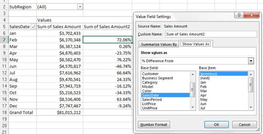
Create a Pivot Table Month-over-Month Variance View for Your Excel Report - dummies

How to unbold Pivot Table row labels - MrExcel Message Board Using Excel 2007, nested Pivot Table rows always seem to bold all but the inner-most row label. Is there a way to unbold all row labels? Displaying in Classic layout, tabular form, without expand/collapse buttons. Showing/Hiding subtotals doesn't seem to matter. I don't recall older versions...

Share :