41 excel chart hide zero labels

How to add data labels from different column in an Excel chart? How to hide zero data labels in chart in Excel? Sometimes, you may add data labels in chart for making the data value more clearly and directly in Excel. But in some cases, there are zero data labels in the chart, and you may want to hide these zero data labels. Here I will tell you a quick way to hide the zero data labels in Excel at once. What is an indexed chart and how to create one using Excel? 09.10.2012 · Indexed Chart Example – Commodity prices in last 5 years. Lets say you are a savvy commodity investor and want to understand how the prices of gold, silver, bananas and coffee have changed since 2007. Now, each of them have a different range of values and comparing all of them in same chart can be very confusing.

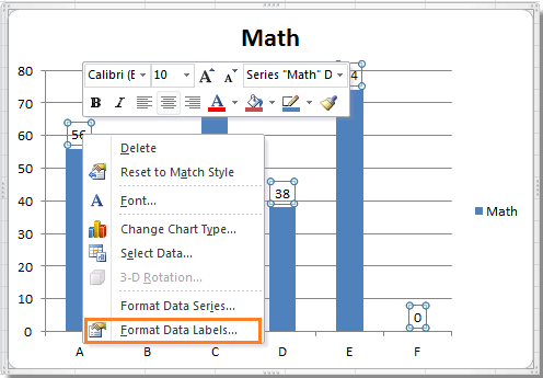
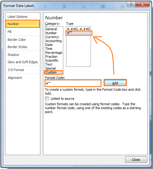
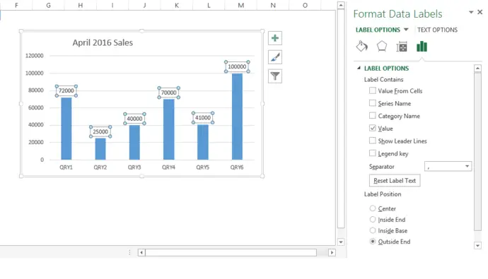
How can I hide 0% value in data labels in an Excel Bar Chart The quick and easy way to accomplish this is to custom format your data label. Select a data label. Right click and select Format Data Labels; Choose the Number category in the Format Data Labels dialog box.

Excel chart hide zero labels

Text Labels on a Horizontal Bar Chart in Excel - Peltier Tech Dec 21, 2010 · In Excel 2003 the chart has a Ratings labels at the top of the chart, because it has secondary horizontal axis. Excel 2007 has no Ratings labels or secondary horizontal axis, so we have to add the axis by hand. On the Excel 2007 Chart Tools > Layout tab, click Axes, then Secondary Horizontal Axis, then Show Left to Right Axis. Make Pareto chart in Excel - Ablebits.com Jun 27, 2018 · The Pareto chart is immediately inserted in a worksheet. The only improvement that you'd probably want to make is to add/change the chart title: Customizing Excel Pareto graph. The Pareto chart created by Excel is fully customizable. You can change the colors and style, show or hide data labels, and more. Design the Pareto chart to your liking Display or hide zero values - support.microsoft.com Select the cells with hidden zeros. You can press Ctrl+1, or on the Home tab, click Format > Format Cells. Click Number > General to apply the default number format, and then click OK. Hide zero values returned by a formula Select the cell that contains the zero (0) value.

Excel chart hide zero labels. How to Hide Zero Values on an Excel Chart - YouTube How to hide zero in chart axis in Excel? - ExtendOffice Click Close to exist the dialog. Now the zero in chart axis is hidden. Tip: For showing zero in chart axis, go back to Format Axis dialog, and click Number > Custom. Select #,##0;-#,##0 in the Type list box. Note: In Excel 2013, you need to click Number tab to expand its option, and select Custom from the Category drop down list, then type ... Actual vs Budget or Target Chart in Excel - Excel Campus 19.08.2013 · Next you will right click on any of the data labels in the Variance series on the chart (the labels that are currently displaying the variance as a number), and select “Format Data Labels” from the menu. On the right side of the screen you should see the Label Options menu and the first option is “Value From Cells”. Click the check box ... How to Hide Zero Values in Excel Pivot Table (3 Easy Methods) - ExcelDemy We can filter the zero values from the Filter field. Just follow these steps to perform this: 📌 Steps. ① First, click on the pivot table that you created from the dataset. ② Now, on the right side, you will see pivot table fields. ③ Now, from the pivot table fields, drag the Quantity and Price into the Filter field.

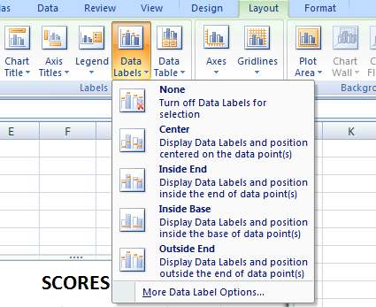
Actual vs Budget or Target Chart in Excel - Variance on ... Aug 19, 2013 · Next you will right click on any of the data labels in the Variance series on the chart (the labels that are currently displaying the variance as a number), and select “Format Data Labels” from the menu. On the right side of the screen you should see the Label Options menu and the first option is “Value From Cells”. Column chart: Dynamic chart ignore empty values | Exceljet To make a dynamic chart that automatically skips empty values, you can use dynamic named ranges created with formulas. When a new value is added, the chart automatically expands to include the value. If a value is deleted, the chart automatically removes the label. In the chart shown, data is plotted in one series. Add or remove data labels in a chart - support.microsoft.com On the Design tab, in the Chart Layouts group, click Add Chart Element, choose Data Labels, and then click None. Click a data label one time to select all data labels in a data series or two times to select just one data label that you want to delete, and then press DELETE. Right-click a data label, and then click Delete. Make Pareto chart in Excel - Ablebits.com 27.06.2018 · The Pareto chart is immediately inserted in a worksheet. The only improvement that you'd probably want to make is to add/change the chart title: Customizing Excel Pareto graph. The Pareto chart created by Excel is fully customizable. You can change the colors and style, show or hide data labels, and more. Design the Pareto chart to your liking

think-cell :: KB0195: How can I hide segment labels for If the chart is complex or the values will change in the future, an Excel data link (see Excel data links) can be used to automatically hide any labels when the value is zero ("0"). Open your data source. Use cell references to read the source data and apply the Excel IF function to replace the value "0" by the text "Zero". Create a think-cell ... Hiding data labels with zero values | MrExcel Message Board Right click on a data label on the chart (which should select all of them in the series), select Format Data Labels, Number, Custom, then enter 0;;; in the Format Code box and click on Add. If your labels are percentages, enter 0%;;; or whatever format you want, with ;;; after it. With stacked column charts, you have to do this for each series ... excel - Hide Category Name From bar Chart If Value Is Zero - Stack Overflow The data typically have some zero values in it that I do not want to show on the chart. I can hide the zero by using custom number format 0;"" but it still leaves the category name and the visible which makes the chart messy to read. Is there any way to accomplish this? enter image description here excel excel-charts Share Improve this question How to Quickly Remove Zero Data Labels in Excel - Medium In this article, I will walk through a quick and nifty "hack" in Excel to remove the unwanted labels in your data sets and visualizations without having to click on each one and delete manually....

Directly Labeling Excel Charts | PolicyViz

Excel - charts - cannot hide the filter buttons in the chart Excel - charts - cannot hide the filter buttons in the chart. Hi, In Excel 2019 I was able to hide the filters buttons in the chart (right-click on the button and choose 'hide all buttons' from the menu) I needed that because I'm filtering via Slicers. Is there a way to hide them in Excel 365? right-click on the filter button won't open any menu.

Removing gaps between bars in an Excel chart - TheSmartMethod.com

Creating a chart with dynamic labels - Microsoft Excel 2016

Hide Series Data Label if Value is Zero - Peltier Tech The trick is to use the value option for the data labels, rather than the series name option. The series names have been replaced by values, and zeros appear where the unwanted series name labels are in the chart above. Then apply custom number formats to show only the appropriate labels.

31 How To Label In Excel - Best Labels Ideas 2020

How to hide zero data labels in chart in Excel? - ExtendOffice In the Format Data Labelsdialog, Click Numberin left pane, then selectCustom from the Categorylist box, and type #""into the Format Codetext box, and click Addbutton to add it to Typelist box. See screenshot: 3. Click Closebutton to close the dialog. Then you can see all zero data labels are hidden.

Excel Vba Change Chart Legend Text - excel dashboard templates how to easily hide zero and blank ...

Column Chart with Primary and Secondary Axes - Peltier Tech 28.10.2013 · The second chart shows the plotted data for the X axis (column B) and data for the the two secondary series (blank and secondary, in columns E & F). I’ve added data labels above the bars with the series names, so you can see where the zero-height Blank bars are. The blanks in the first chart align with the bars in the second, and vice versa.

how to make a excel graph.

Create Dynamic Chart Data Labels with Slicers - Excel Campus 10.02.2016 · Typically a chart will display data labels based on the underlying source data for the chart. In Excel 2013 a new feature called “Value from Cells” was introduced. This feature allows us to specify the a range that we want to use for the labels. Since our data labels will change between a currency ($) and percentage (%) formats, we need a ...

How to hide zero data labels in chart in Excel?

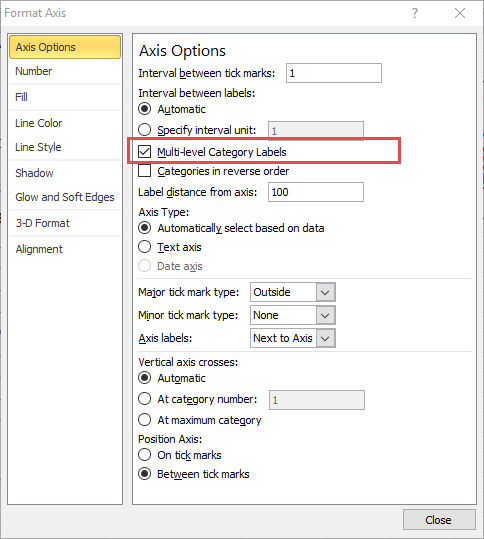
How to hide points on the chart axis - Microsoft Excel 2016 Excel 2016. Sometimes you need to omit some points of the chart axis, e.g., the zero point. This tip will show you how to hide specific points on the chart axis using a custom label format. To hide some points in the Excel 2016 chart axis, do the following: 1. Right-click in the axis and choose Format Axis... in the popup menu:

Need help making labels on a graph with format code : excel

How to hide points on the chart axis - Microsoft Excel 365 - OfficeToolTips The first applies to positive values, the second to negative values, and the third to zero (for more details see Conditional formatting of chart axes). 3. Click the Add button. See also this tip in French: Comment masquer des points sur l'axe du graphique.

Label Specific Excel Chart Axis Dates • My Online Training Hub

How to hide "0" in chart axis [quick tip] - Chandoo.org Here is a handy little trick to do just that: Select the axis and press CTRL+1 (or right click and select "Format axis") Go to "Number" tab. Select "Custom". Specify the custom formatting code as #,##0;-#,##0;; Press "Add" if you are using Excel 2007, otherwise press just OK. That is all.

How to hide zero data labels in chart in Excel?

Text Labels on a Horizontal Bar Chart in Excel - Peltier Tech 21.12.2010 · In Excel 2003 the chart has a Ratings labels at the top of the chart, because it has secondary horizontal axis. Excel 2007 has no Ratings labels or secondary horizontal axis, so we have to add the axis by hand. On the Excel 2007 Chart Tools > Layout tab, click Axes, then Secondary Horizontal Axis, then Show Left to Right Axis.

How to hide zero value rows in pivot table?

Highlight Max & Min Values in an Excel Line Chart - Xelplus We will begin by creating a standard line chart in Excel using the below data set. Click anywhere in the data and select Insert (tab)-> Charts (group) -> Insert Line or Area Chart (button)-> Line with Markers (top row, second from right).. Using the newly created line chart, if we were to manually change the color of the highest value on the line, we would perform the following …

33 How To Label A Pie Chart In Excel - Labels 2021

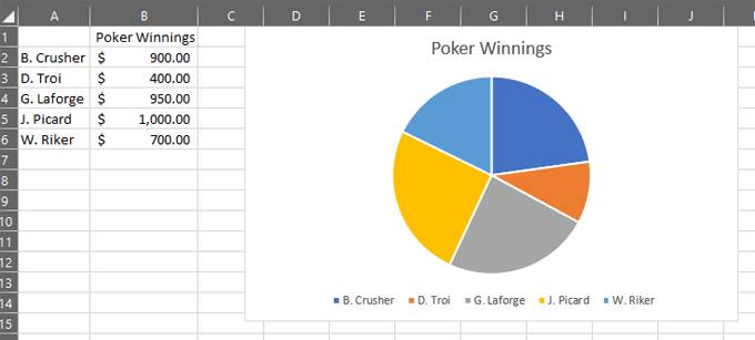
Hide Category & Value in Pie Chart if value is zero 1. Select the axis and press CTRL+1 (or right click and select "Format axis") 2. Go to "Number" tab. Select "Custom". 3. Specify the custom formatting code as #,##0;-#,##0;; 4. Press "Add" if you are using Excel 2007, otherwise press just OK. Any solution for Hiding Category also from chart if the value is zero and its display ...

Do My Excel Blog: How to hide the zero percent labels in an Excel pie chart

Creating a chart in Excel that ignores #N/A or blank cells My chart has a merged cell with the date which is my x axis. The problem: BC26-BE27 are plotting as ZERO on my chart. enter image description here. I click on the filter on the side of the chart and found where it is showing all the columns for which the data points are charted. I unchecked the boxes that do not have values. enter image ...

SSRS Charts with Data Tables (Excel Style) | Some Random Thoughts

Hide data labels with low values in a chart - Excel Help Forum Hide data labels with low values in a chart. To hide chart data labels with zero value I can use the custom format 0%;;;, But is there also a possibility to hide data labels in a chart with values lower that a certain predefined number (e.g. hide all labels < 2%)? Register To Reply. 03-29-2013, 12:06 PM #2. Andy Pope.

Formula Friday - Using Formulas To Add Custom Data Labels To Your Excel Chart - How To Excel At ...

Creating a chart in Excel that ignores #N/A or blank cells I am attempting to create a chart with a dynamic data series. Each series in the chart comes from an absolute range, but only a certain amount of that range may have data, and the rest will be #N/A.. The problem is that the chart sticks all of the #N/A cells in as values instead of ignoring them. I have worked around it by using named dynamic ranges (i.e. Insert > Name > Define), …