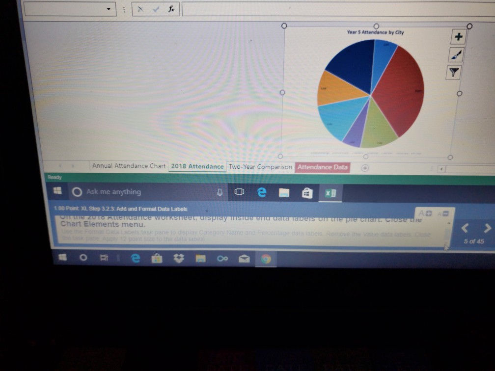
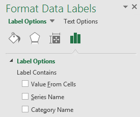
40 use the format data labels task pane to display category name and percentage data labels
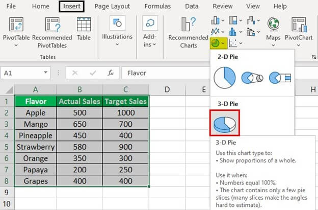
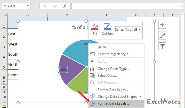
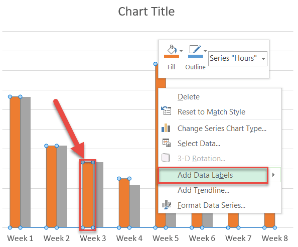
Excel Module 4 Flashcards | Quizlet you want to show the percentages only, not their numerical values.in the task pane, in the label contains section, click the value check box to deselect it.excel removes the numerical values from the data labels.in the label position section, click the inside end option button to select it.excel moves the data labels to the inside end position.in … Excel 3-D Pie charts - Microsoft Excel 2016 - OfficeToolTips 2. On the Insert tab, in the Charts group, choose the Pie button: Choose 3-D Pie. 3. Right-click in the chart area, then select Add Data Labels and click Add Data Labels in the popup menu: 4. Click in one of the labels to select all of them, then right-click and select Format Data Labels... in the popup menu: 5.
Change the format of data labels in a chart To get there, after adding your data labels, select the data label to format, and then click Chart Elements > Data Labels > More Options. To go to the appropriate area, click one of the four icons ( Fill & Line, Effects, Size & Properties ( Layout & Properties in Outlook or Word), or Label Options) shown here.
Use the format data labels task pane to display category name and percentage data labels
How to create a chart with both percentage and value in Excel? In the Format Data Labels pane, please check Category Name option, and uncheck Value option from the Label Options, and then, you will get all percentages and values are displayed in the chart, see screenshot: 15. Succeeding in Business with Microsoft Excel 2013: A ... Debra Gross, Frank Akaiwa, Karleen Nordquist · 2013 · ComputersYou can use this task pane to change the label options to display the series name, category name, value, and/or percentage. You can also change the data ... Format Chart Axis in Excel - Axis Options Analyzing Format Axis Pane. Right-click on the Vertical Axis of this chart and select the "Format Axis" option from the shortcut menu. This will open up the format axis pane at the right of your excel interface. Thereafter, Axis options and Text options are the two sub panes of the format axis pane.
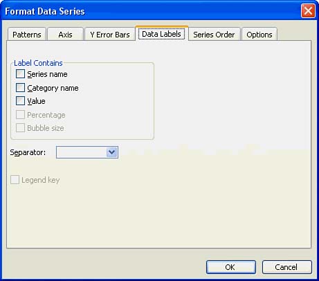
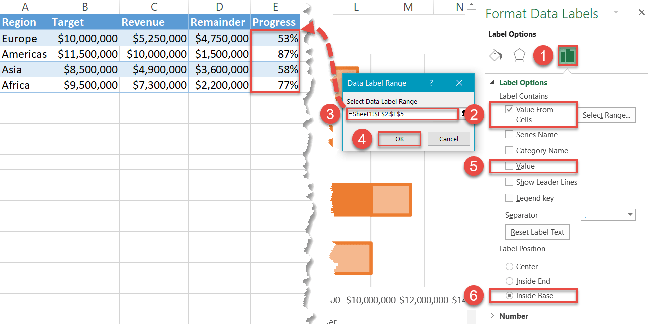
Use the format data labels task pane to display category name and percentage data labels. › 38307875 › Advanced_excel_tutorial(PDF) Advanced excel tutorial | Adeel Zaidi - Academia.edu There are many options available for formatting of the Data Labels in the Format Data Labels Task Pane. Make sure that only one Data Label is selected while formatting. 29 Advanced Excel Step 9: In Label Options →Data Label Series, click on Clone Current Label. This will enable you to apply your custom Data Label formatting quickly to the ... Add or remove data labels in a chart - support.microsoft.com Right-click the data series or data label to display more data for, and then click Format Data Labels. Click Label Options and under Label Contains, select the Values From Cells checkbox. When the Data Label Range dialog box appears, go back to the spreadsheet and select the range for which you want the cell values to display as data labels. › excel_dax › excel_dax_quickExcel DAX - Quick Guide - tutorialspoint.com Renaming a Calculated Field in the Data Model. You can change the name of a calculated field in the Data Table either in Data View or Diagram View. Renaming a Calculated Field in the Data View. Click the calculated field in the table in data view of the Data Model. Select the calculated field name in the formula bar – to the left side of :=. How do you format data series in Excel? - FAQ-ALL To format data labels in EÎl , choose the set of data labels to format . To do this, click the " Format " tab within the "Chart Tools" contextual tab in the Ribbon. Then select the data labels to format from the "Chart Elements" drop-down in the "Current Selection" button group.
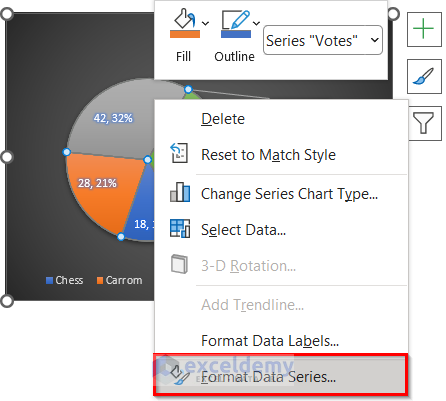
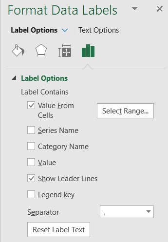
Filtering charts in Excel | Microsoft 365 Blog Select the chart, then click the Filter icon to expose the filter pane. From here, you can filter both series and categories directly in the chart. For example, hover over Fruit Pear and see how the category is highlighted. To get the same view we created in our earlier chart, we'll hide the Cost/lb column. Under Series, uncheck Cost/lb, and ... Format Data Labels in Excel- Instructions - TeachUcomp, Inc. To format data labels in Excel, choose the set of data labels to format. To do this, click the "Format" tab within the "Chart Tools" contextual tab in the Ribbon. Then select the data labels to format from the "Chart Elements" drop-down in the "Current Selection" button group. A data label is descriptive text that shows that - Course Hero To format the data labels - Double click a data label to open the Format Data Labels task pane. Click the Label Options Icon. Click Label Options to customize the labels, and complete any of the following steps: Select the Label Contains options. The default is Value, but you might want to display additional label contents, such as Category ... In the format data labels pane under label contains - Course Hero In the Format Data Labels pane, under Label Contains, click to select the Category Name check box. Click to deselect the Value check box. Click to select the Percentage check box. Click to deselect the Show Leader Lines check box. Under Label Position, select the Center option. Click the Close button.
How to: Display and Format Data Labels - DevExpress In particular, set the DataLabelBase.ShowCategoryName and DataLabelBase.ShowPercent properties to true to display the category name and percentage value in a data label at the same time. To separate these items, assign a new line character to the DataLabelBase.Separator property, so the percentage value will be automatically wrapped to a new line. Enhanced Microsoft Excel 2013: Comprehensive Steven M. Freund, Mali Jones, Joy L. Starks · 2015 · Business & EconomicsTap or click the X Rotation up arrow (Format Chart Area dialog box) until the X ... Set Data Labels to show the Category Name, Percentage, and Leader Lines. How to show data label in "percentage" instead of - Microsoft Community Select Format Data Labels Select Number in the left column Select Percentage in the popup options In the Format code field set the number of decimal places required and click Add. (Or if the table data in in percentage format then you can select Link to source.) Click OK Regards, OssieMac Report abuse 8 people found this reply helpful · Advanced Excel - Quick Guide - tutorialspoint.com The Format Data Label Task Pane appears. There are many options available for formatting of the Data Label in the Format Data Labels Task Pane. Make sure that only one Data Label is selected while formatting. Step 9 − In Label Options → Data Label Series, click on Clone Current Label. This will enable you to apply your custom Data Label ...
How to Make a Pie Chart in Excel (5 Suitable Examples)
admx.helpAllow Basic authentication - admx.help Use DNS name resolution when a single-label domain name is used, by appending different registered DNS suffixes, if the AllowSingleLabelDnsDomain setting is not enabled. Use DNS name resolution with a single-label domain name instead of NetBIOS name resolution to locate the DC; Allow cryptography algorithms compatible with Windows NT 4.0

How to make a pie chart in Excel
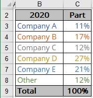
How to make a pie chart in Excel - Ablebits.com Right click any slice on your chart, and select Format Data Labels… in the context menu. On the Format Data Labels pane, select either the Value or Percentage box, or both as in the following example. Percentages will be calculated by Excel automatically with the entire pie representing 100%. Explode a chart pie or pull out individual slices
How to get an Excel chart to display percentages of each ...
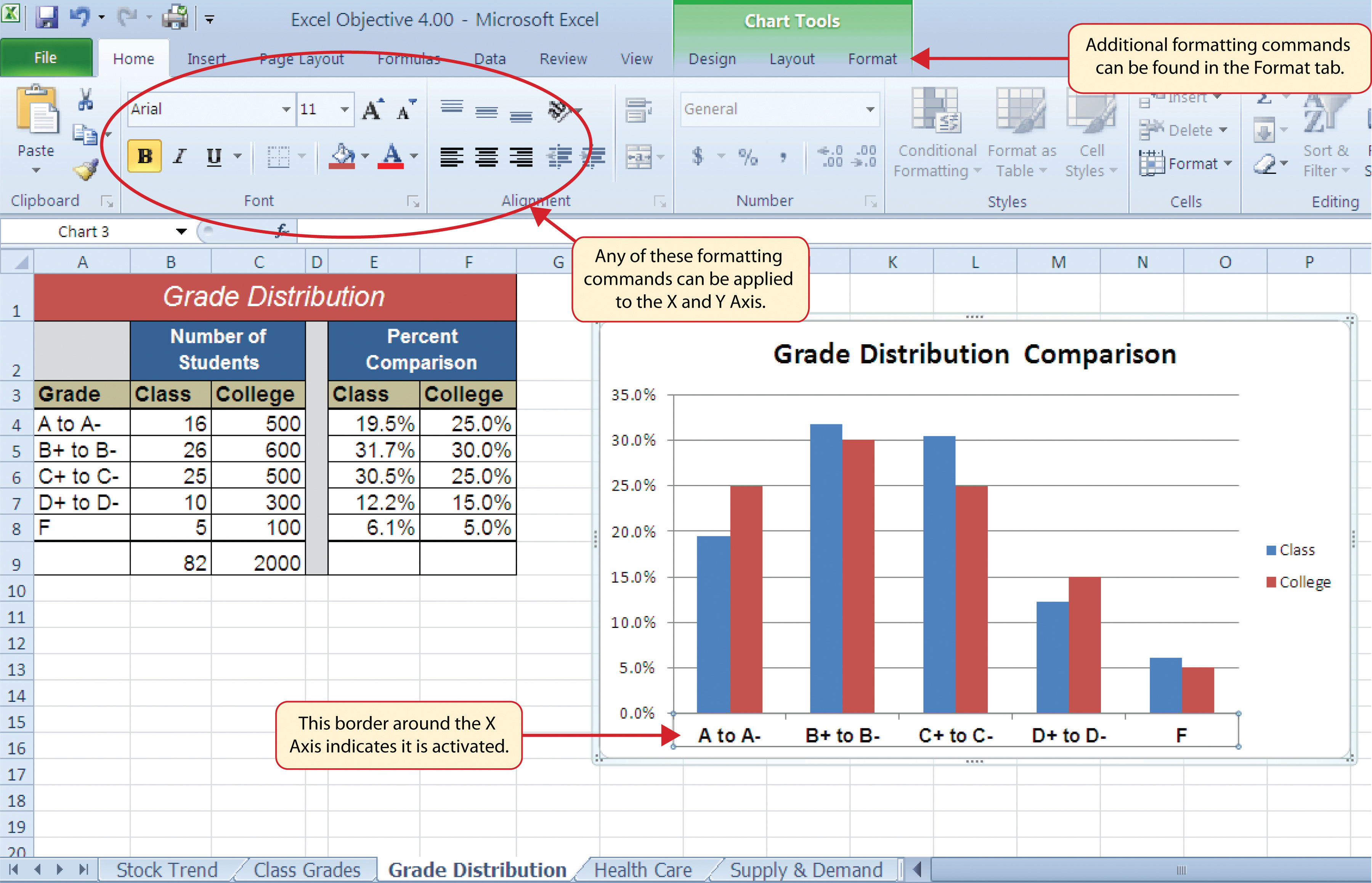
Solved 7 Add data labels for the % of Month line. Position | Chegg.com Apply 11 pt font size to the category axis, value axis, and the legend for the bar chart. 14. Use the Axis Options to display the value axis in units of Thousands, set the Major Units to 500, apply the Number format with 1 decimal place for the bar chart. Use the Axis Options to format the category axis so that the category labels are in ...

How to show percentages on three different charts in Excel ...
How to use data labels - Exceljet When first enabled, data labels will show only values, but the Label Options area in the format task pane offers many other settings. You can set data labels to show the category name, the series name, and even values from cells. In this case for example, I can display comments from column E using the "value from cells" option.
Presenting Data with Charts
Custom Number Format in Pie Chart | MrExcel Message Board Sep 2, 2016. #3. - Create a table as shown below. - With Excel 2013 or later, specify the desired range to populate the data labels: format data labels task pane>value from cells>select range. - Important: depending on your regional settings, use commas or dots in the appropriate places at the formula. Charts.

How to create a chart with both percentage and value in Excel?
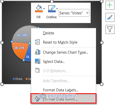
4.2 Formatting Charts - Beginning Excel, First Edition Right click and select Format Data Series to open up the Format Data Series pane. Click the Fill and Line (paint bucket) button to bring up the Fill and Border group of commands. Click the word Fill (if needed) to expand the list of Fill options. Select Pattern Fill. Then select 30% (fifth column, top row).

How to create a chart with both percentage and value in Excel?
Work Distribution Report with Hours and Percentages Now right-click the doughnut and select Format Data Labels; then select Percentage, Category Name, Value, Legend Key, Show Leader Lines in the Format Data Labels pane (LABEL OPTIONS), and also ...
Presenting Data with Charts
Solved step by step instruction 2 A pie chart is an | Chegg.com Use the Insert tab to create a pie chart from the Question: step by step instruction 2 A pie chart is an effective way to visually illustrate the percentage of the class that earned A, B, C, D, and F grades. Use the Insert tab to create a pie chart from the This problem has been solved! See the answer step by step instruction Expert Answer

How to insert data labels to a Pie chart in Excel 2013
Excel bar chart with conditional formatting based on MoM change Use the chart skittle to select Data Labels and select More Options to display the Data Labels task pane. Check the Value From Cells checkbox and select the cells containing the custom labels for this series, cells E16 to E20 in this example. It is important to select the entire range because the label can move based on the data.
Change the format of data labels in a chart
Shelly Cashman Series Microsoft Office 365 & Excel 2016: ... Steven M. Freund, Joy L. Starks, Eric Schmieder · 2016 · Business & EconomicsClick More Options to display the Format Data Labels task pane. ... click to display check marks in the Category Name, Percentage, and 'Show Leader Lines' ...
Excel 3-D Pie charts - Microsoft Excel 365
admx.helpBlock signing into Office Default file format; Disable the Office Start screen for Access; Do not prompt to convert older databases; List of managed add-ins; Never cache data; Personal templates path for Access; Show custom templates tab by default in Access on the Office Start screen and in File | New; Use Access 2007 compatible cache; Tools | Security. Workgroup ...
Pie Charts in Excel - How to Make with Step by Step Examples
How to show percentages on three different charts in Excel To convert the calculated decimal values to percentages, right-click on the selected cells and click Format Cells. Alternatively, press CTRL+1 on the keyboard to open the Format Cells dialogue box. 3. In the Format Cells dialogue box, make sure that the Number tab is selected and in the Category list select Percentage.
Excel bar chart with conditional formatting based on MoM ...
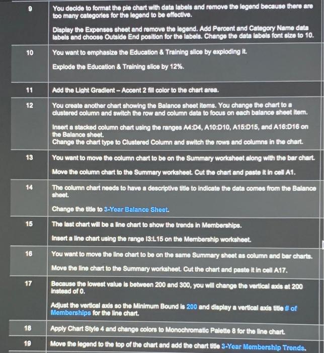
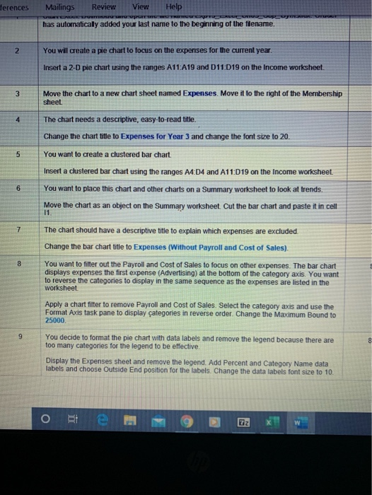
Excel chapter 3: grader project | Management homework help - SweetStudy Add Percent and Category Name data labels and choose Outside End position for the labels. Change the data labels font size to 10. 810You want to emphasize the Education & Training slice by exploding it. Explode the Education & Training slice by 12%. 211Add the Light Gradient - Accent 2 fill color to the chart area.
How to Make Pie Chart with Labels both Inside and Outside ...
support.unicomsi.com › manuals › intelligenceUNICOM Intelligence Using the variables pane with hierarchical data. ... Viewing category full names for use in a filter in a DMS file ... Converting data to the required format
Is it possible to adjust the data label text box dimension in ...
Exp19_excel_ch03_cap_gym | Computer Science homework help You decide to format the pie chart with data labels and remove the legend because there are too many categories for the legend to be effective. Display the Expenses sheet and remove the legend. Add Percent and Category Name data labels and choose Outside End position for the labels. Change the data labels font size to 10.

How to show percentages on three different charts in Excel ...
Display the percentage data labels on the active chart. - YouTube Display the percentage data labels on the active chart.Want more? Then download our TEST4U demo from TEST4U provides an innovat...
Question | Chegg.com
doc.igrafx.com › doc › tutorialsiGrafx Client Tutorial - iGrafx Process360 Live Click the Format tab and change the Display As setting to Graph. Click the Graph Style button. Click the Line graph button. Click OK to save changes and close the Graph Control dialog box. Click OK to save and close the Edit Report Element dialog box. Your report element is changed to a line graph. Make a copy to show the data in table format:
![Ultimate Guide to Creating Charts in Excel [2022] - onsite ...](https://www.onsite-training.com/wp-content/uploads/2020/05/Pie-5.jpg)
Ultimate Guide to Creating Charts in Excel [2022] - onsite ...
cs 385 exam 3 Flashcards | Quizlet data tab, subtotal, click at each change in: select area, unselect replace current subtotals, click ok Collapse the table to show the grand totals only. click 1 at top left corner Expand the table to show the grand and discipline totals. click 2 at top left corner Use the Auto Outline feature to group the columns.

Add or remove data labels in a chart
quizlet.com › 343637424 › misc-211-final-flash-cardsMISC 211 Final Flashcards | Quizlet On the Chart Tools Format tab, in the Current Selection group, click the Format Selection button to open the Format Data Point task pane. In the Point Explosion box, type 50 and press Enter. Filter the chart so the lines for Dr.Patella and John Patterson are hidden.

Excel Charts - Aesthetic Data Labels
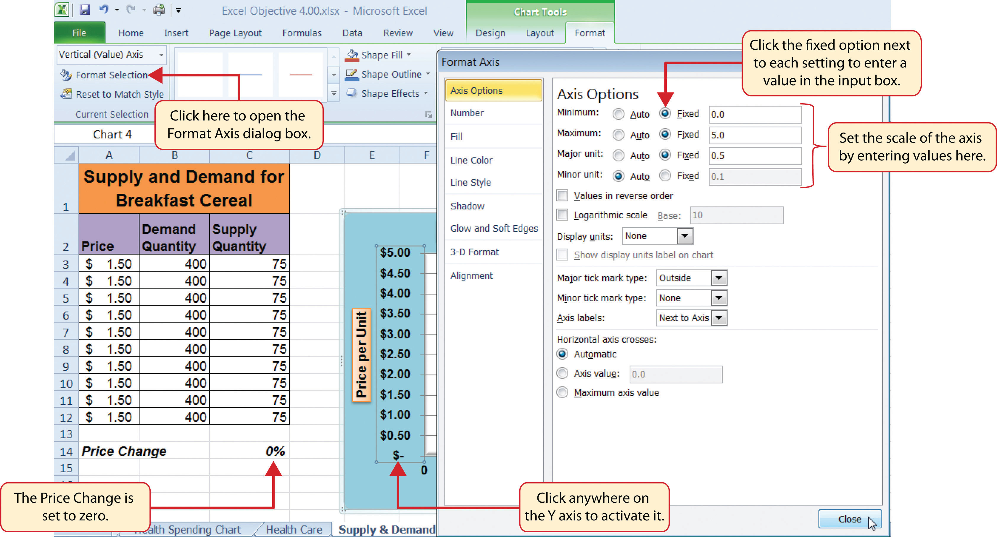
Format Chart Axis in Excel - Axis Options Analyzing Format Axis Pane. Right-click on the Vertical Axis of this chart and select the "Format Axis" option from the shortcut menu. This will open up the format axis pane at the right of your excel interface. Thereafter, Axis options and Text options are the two sub panes of the format axis pane.

Change the format of data labels in a chart
Succeeding in Business with Microsoft Excel 2013: A ... Debra Gross, Frank Akaiwa, Karleen Nordquist · 2013 · ComputersYou can use this task pane to change the label options to display the series name, category name, value, and/or percentage. You can also change the data ...
Analyzing Data with Tables and Charts in Microsoft Excel 2013 ...
How to create a chart with both percentage and value in Excel? In the Format Data Labels pane, please check Category Name option, and uncheck Value option from the Label Options, and then, you will get all percentages and values are displayed in the chart, see screenshot: 15.

Custom data labels in a chart

How to Use Cell Values for Excel Chart Labels
Is it possible to adjust the data label text box dimension in ...
Working with Charts :: Hour 12. Adding a Chart :: Part III ...
Solved Step Instructions Start Excel. Download and open the ...

Display Customized Data Labels on Charts & Graphs
How to Create Progress Charts (Bar and Circle) in Excel ...
How to Create a Timeline Chart in Excel - Automate Excel

Change the format of data labels in a chart
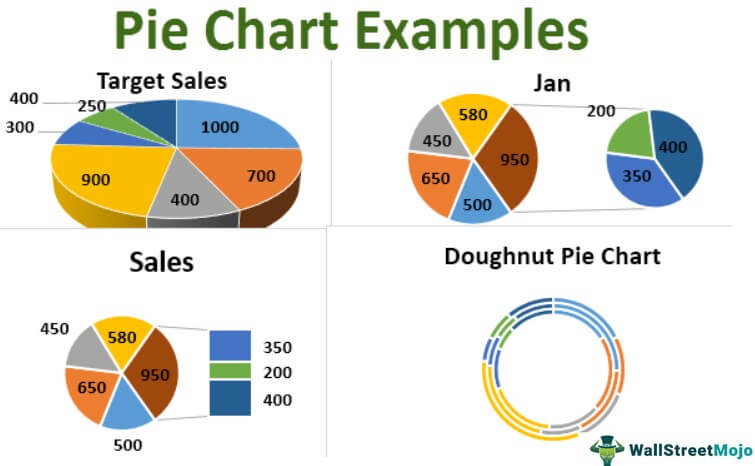
Pie Charts in Excel - How to Make with Step by Step Examples
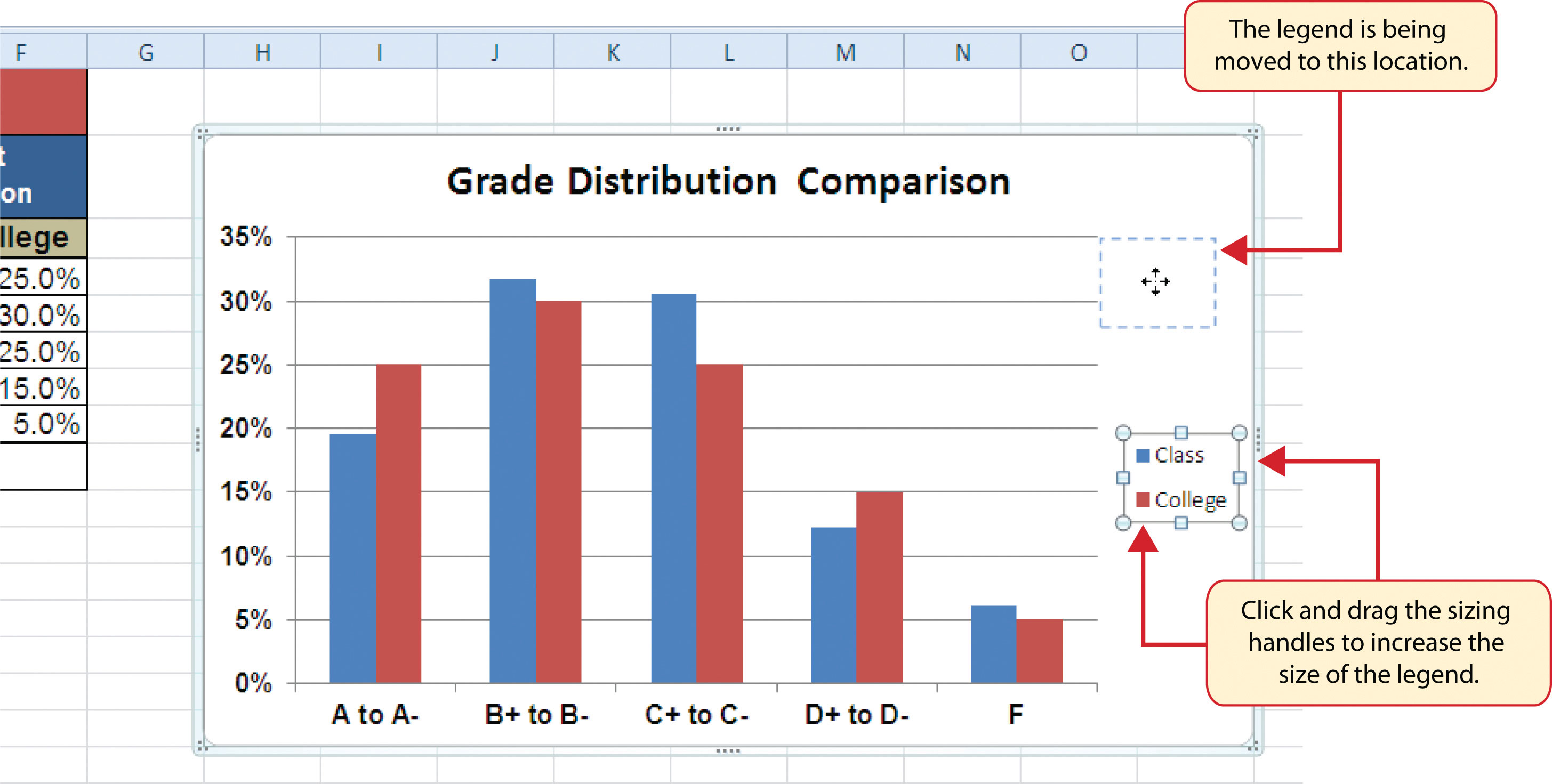
Presenting Data with Charts

Formatting Data Labels
Creating a Pie Chart: IU Only: Files: Excel 2016: Charts and ...

How to make a pie chart in Excel

Change the format of data labels in a chart
Please SHOW me how to do steps 8-22 on excel or at | Chegg.com
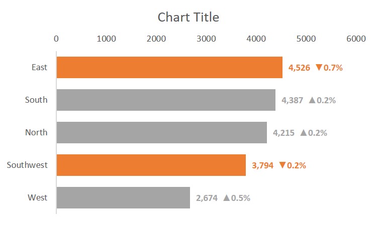
Excel bar chart with conditional formatting based on MoM ...
How to Make a Pie Chart in Excel (5 Suitable Examples)
Post a Comment for "40 use the format data labels task pane to display category name and percentage data labels"